The Shivering Universe
As galaxies collide, the Universe shivers.
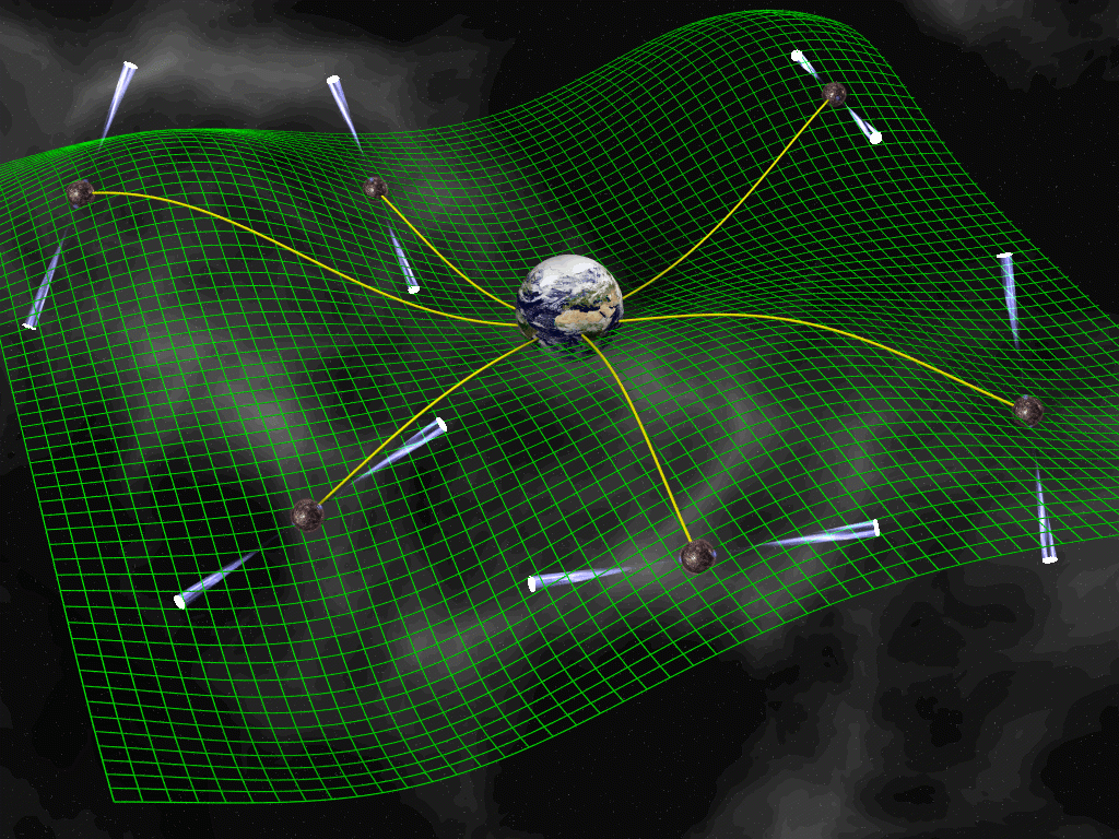 A pulsar timing array, or PTA.
On the morning of September 14th, 2015, two LIGO observatories, one in Hanford and the other in Livingston, detected the gravitational waves from the merger of two massive black holes. Labelled GW150914 (the numbers correspond to the date of discovery), this detection changed the face of astronomy forever. No longer were astronomers dependent on electromagnetic radiation to peer into the mysteries of the cosmos. Now, they could feel it shiver, as neutron stars, black holes and galaxies merged, tore each other apart and became one. Soon, scientists realised that they could use the very Universe itself as an interferometer, for it had already given us the tools: pulsars. Recall that pulsars are characterised by their period, $\mathbf{P}$ and period derivative, $\mathbf{\dot P}$, which we plot in a $\mathbf{P - \dot P}$ diagram. Pulsars with low $\mathbf{P}$ and $\mathbf{\dot P}$ are known as millisecond pulsars (MSPs); due to the low values of both parameters, they are very stable rotators, with their spin having the same precision as atomic clocks. In other words, pulsars are clocks! But how do we use these (very precise) clocks to detect gravitational waves?
pulsar timing – n. the unambiguous accounting of each and every rotation of a neutron star
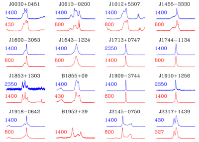
Pulsars are detected through their radio emission; each time their beam(s) crosses the line of sight between them and Earth, our radio telescopes detect a pulse. But often, these pulses are buried in noise; those random wiggles that you often see in real data (or the black and white freckles on the TV screen when the cable is out). And to recover the pulse, the data is often cut into segments of time equal to the pulsar period, and then added together; this process (if you read my previous articles) is known as folding. After folding, we have an average profile of the pulse; if the pulsar is a clock, this is our tick, heard back on Earth. We hear the ticks, make a model that can replicate those ticks and then predict the arrivals of later ticks, hoping that we have maintained phase connection (more on that in a minute). This is the process of pulsar timing; we are trying to account for every rotation the neutron star makes. The model we created is called a timing solution; the more data we have, the better this model will be. But I have glossed over something very important: what is meant by “phase connection“?
Lets think of a real-life example of phase connection: you are preparing for an exam. You have not slept the whole night and are barely keeping up with what’s going on in the book. Suddenly, you fall asleep and then wake up after a while, frantic, looking for your phone as if your life depended on it so that you can check the time. Why is that? When you were awake, you could account for the passing of every minute as you studied; think of those minutes as the rotations, the ticks of the pulsar. When you suddenly slept and woke up, you lost track of time; in other words, you lost phase connection! You could no longer account for every minute. For all you knew, you might have missed the test itself! That’s what phase connection implies: are you still in step with the ticks? Did you miss any? If everything goes as it should, you probably didn’t, and your timing solution is good to go.
Each tick you hear is known as a time-of-arrival (TOA) measurement. But if you actually want to time a pulsar, you would want to be present at the pulsar’s location itself. Why is that? If you recall, the interstellar medium (ISM), being a plasma, disperses the pulsar signal, adding to your problems. The pulsar itself could be moving (particularly since most MSPs are in binary systems). And the Earth moves around the Sun, and the Sun moves around the galaxy and so on. All these movements (and dispersion) add time delays to your TOAs. That is, you don’t really hear the tick when you should; it is a little late and, for a clock that is supposed to be as precise as an atomic clock, even a few micro- or milliseconds of delay is bad. TOAs are, after all, merely proxies for what you actually want to measure: the passage of time of a single, fixed point on a neutron star.
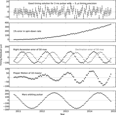
To convert your proxies into what you really want, you calculate and get rid of each of those time delays, one by one. In the end, what you obtain is a residual: (your prediction of the tick) – (when the tick actually arrived). These timing residuals should, ideally, be like white noise: completely random, with amplitudes that are independent of frequency (what is known as a flat power spectrum). If you messed up, your residuals would look very different, as the figure below shows.
Timing models can be very precise, with values that are good to up 10s of decimal places (see below). But I have still not answered the second question: how do you use these ultra-precise clocks to detect ripples in space-time? Think of an interferometer, like LIGO. It can be thought of as a two-way timing device: you send out a light beam along one arm, it comes back, and you time it. If it took longer than expected of light, the space must have stretched in between, and you have detected a gravitational wave. Of course it is more complicated than it sounds: instead of using a clock to time it, another light beam, sent out in a perpendicular direction is used. When they meet, they interfere destructively at the “dark port“. If a gravitational wave passes through, each of the arms would alternatively be stretched and compressed (while one arm stretches, the other compresses). They would no longer arrive at the same times as before, and would interfere constructively. You will see flickers of light at the “dark port” and declare that you have detected a gravitational wave.
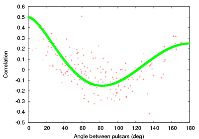
But with pulsars, you use it as a one-way timing device: the pulsar sends out a pulse, and you time it. If it arrived at the right time (according to your timing model), then there is nothing. But if the pulse is late, you may have detected a gravitational wave. This is the principle behind the construction of a Pulsar Timing Array, or PTA: use many pulsars, time them and build their timing models. After you have got the timing models, you compare all the residuals with one another. But what are you looking for? If a gravitational wave did pass your pulsars in the PTA, you would see a correlation (or anti-correlation); in other words, you would see that the residuals all vary in either the same way, or in the exactly opposite way. If you see that, you may have detected gravitational waves. This correlation-anti-correlation signature you are looking for is known as the Hellings and Down curve and is shown below. It gives you the expected correlation (negative values imply an anti-correlation) between a pair of pulsars based on the angle between them. You calculate this for all the pulsar pairs in your PTA.
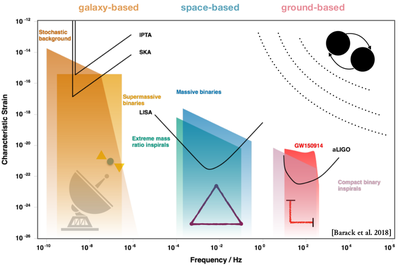
If you have been following all the arguments up till now, you may have noticed another thing I have glossed over: I did not tell you where the gravitational waves are coming from. Are they from black hole mergers? Neutron star mergers? Or something else entirely? The PTA, as it turns out, is the wrong kind of “instrument” to detect the kind of mergers detected by LIGO. What it is really detecting is the merger of entire galaxies. As galaxies merge, so do the supermassive black holes (SMBHs) at their centres, and any other, smaller black holes (inside the galaxies) may merge too. The whole event gives out quite a lot of ripples. Since there are about a 100 billion galaxies in the Universe, and we expect one to merge every 10 billion years, we expect 10 mergers per year. We can estimate, using this rate, that the number of mergers of supermassive black holes would be of the order of a trillion (1 with twelve zeros after it). All of these mergers, happening randomly all over the universe, form a background of ripples that is ever present. This is what the PTAs are out to detect, since their observation times are of the order of several weeks to several years, and the frequency of these ripples is of the order of a few nano- to micro-Hertz (frequency = $\mathbf{f \sim \frac{1}{1 , week} , - , \frac{1}{1 , yr} \approx 10^{-6} - 10^{-9}}$ Hz).
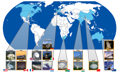
The International Pulsar Timing Array (IPTA) comprises of radio telescopes from 10 countries (including the GMRT and Ooty Telescope arrays from India) that are detecting and timing as many MSPs as they can get their hands on. The IPTA has several country-specific chapters: the European Pulsar Timing Array (EPTA), the North American Nanohertz Observatory for Gravitational Waves (NANOGrav), and the Parkes Pulsar Timing Array (PPTA) as well as the emerging efforts like the Indian Pulsar Timing Array (InPTA), South African Pulsar Timing Array and the Chinese Pulsar Timing Array. The IPTA represents the growing trend in the scientific community of international collaborations (examples of other such collaborations are LIGO, ITER (International Thermonuclear Experimental Reactor), the TMT (Thirty Meter Telescope) and others). Such collaborations help scientists accomplish greater goals in lesser time than they could on their own. It also ensures that, in a time where more and more disciplines are crossing over one another, scientists across fields can help each other out. Additionally, in these politically troubled times, it also fosters friendly relations between different countries.
While they are still waiting for detections, they have slowly pulled the noose on the limits of the gravitational wave amplitudes that they could have detected but didn’t, using their 11-year dataset. This constraints models of galaxy evolution and galactic mergers. And PTAs can give out a lot of unexpected secondary science, from detecting variations in the solar wind to helping in navigation of space missions. Look out for news on detections (or no detections, which would be a surprising result in itself) by the year 2022, when the IPTA datasets will cover their expected signal range.
Meanwhile, the Universe shivers.
References and Further Reading:
- Pulsar timing arrays: the promise of gravitational wave detection, Lommen, A., Rep. Prog. Phys., 78, 124901 (2015): A review of PTAs and their potential for detecting gravitational waves by Andrea Lommen.
- The NANOGrav 11 yr Data Set: Solar Wind Sounding through Pulsar Timing, Madison, D. R., et. al., ApJ, 872, 150 (2019): An analysis of the NANOGrav 11 yr Data Set to study variations in solar wind. Pulsars are accurate probes for the electron density of the ISM, through the time delays introduced by dispersion. Thus, a study of the timing residuals can tell you a lot about variations of electron density, including those caused by the solar wind.
- Upper Limits on the Isotropic Gravitational Radiation Background From Pulsar Timing Analysis, Hellings, R. W. and Downs, G. S., ApJ, 265: L39-L42 (1983): The original paper where the Hellings and Downs curve was first presented.
- Discovery of a Pulsar in a Binary System, Hulse, R. A. and Taylor, J. H., ApJ, 195: L51-53 (1975) and A New Test Of General Relativity: Gravitational Radiation and the Binary Pulsar PSR 1913+16, Taylor, J. H. and Weisberg, J. M., ApJ, 253: 908-920 (1982): The original discovery and analysis papers for the Hulse-Taylor binary system, where study of the gradual decline of the orbit period of the system through the timing residual of the pulsar provided the first indirect confirmation of gravitational waves. The predictions of General Relativity for, and observations of, the orbital period decline matched to unprecedented accuracy, leading to Hulse and Taylor winning the Nobel Prize in Physics in 1993.
- The IPTA 2019 lectures are available here.
- Also check out the Gravitational Wave Calculator here, where you can populate the Universe with your own supermassive black holes and simulate the residuals you will get from a PTA.
Ujjwal Panda
i am an astrochemist and a radio/pulsar astronomer.